The following model is designed as a tutorial showing basic capabilities of QGIS/SEXTANTE in ecological modeling. The data used is from the Sobibor Forest District, southern Poland (data available by the courtesy of Polish State Forests). It represents a case where we would like to find what factors are influencing certain kind of choices like animals habitat selection, nesting places or breeding places. There are many variables that can be taken into consideration, but for the sake of this tutorial only two were taken into account – the distance from the rivers and the forest site types.
1. Setting the model inputs
Locations – investigated points, such as observations, nest locations, breeding locations etc.
Line features – like roads, railways, rivers, etc.
Habitat type – land use types, such as fields, swamps, forests etc. In this case forest types
Habitat type field –this is the table field which describes habitat types
Habitat extent – limits the area for the analysis.
2. Importing layers
Use the standard QGIS Add vector layer dialog.
3. Creating random point layer
To compare the habitat used with available habitat, a point layer generated randomly is created. The GRASS v.random function can be used, in this case to create a new layer with 150 points.
4. Rasterizing rivers layer and creating a distance raster
While dealing with line features, it may be a good idea to analyze the distance from them. The GRASS v.to.rast.value function can be used. The cell size has been left with its default value. Then a distance map can be created with GRASS r.grow.distance function, with a cell size set to 50.
Note: Also SAGA Shapes to Grid command can be used for rasterizing.

5. Adding habitat values to the points.
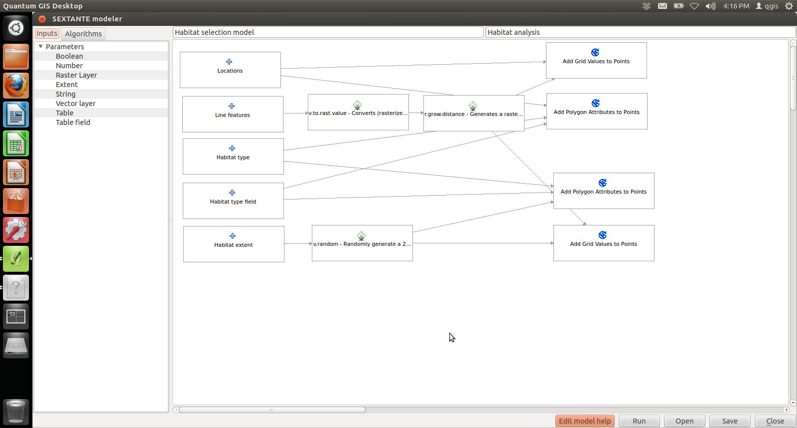
SAGA Add Polygon Values to Points can be used to “transfer” polygon data to point data, in this case from the habitat layer to the points one. In a similar way SAGA Add Grid Values to Points can be used to “transfer” raster data to points data, in this case we use to transfer the value of the distance map to the points one. In both cases there was no need to create appropriate table fields since SAGA created them automatically. The first part of the model is finished and it looks like:
6. Performing statistical analysis
The next step is to import attribute table into the spreadsheet and editing it. A “Use” column with values “1” for the location points points and “0” for the randomly generated points is created. After that the unnecessary columns are removed and results are later imported into R. See 12).
7. Rasterizing habitat layer
GRASS v.to.rast.attr function is used, based on the type_num field which has been previously updated, so each forest site type has been assigned different value from 1 to 15 corresponding with the number of site types. Non-forest areas are given the 0 value. The Field Pyculator QGIS plug-in to fill the type_num field. Then the raster can be reclassified, so every site type represents a corresponding suitability factor. GRASS r.reclass can be used for this operation.
Note: SAGA Shapes to Grid can also be used for rasterizing, and QGIS Create equivalent numerical field function can be used instead of Field Pyculator.
8. Reclassifying rivers distance raster
To fit the rivers raster layer into the final calculations the SAGA Grid Calculator tool is used. The formula for is:
a/1000 * habitat suitability value for rivers
The 1000 factor is used change meters into kilometers.
Note: The same operation can be done in GRASS r.mapcalculator
9. Creating a habitat suitability raster.
GRASS r.mapcalculator is used to finally compute the resulting layer. The formula is simple
a(habitat raster) + b(rivers raster)
10. Rescaling raster
Another step is to rescale final raster with GRASS r.rescale, so it would represent the suitability values in a percentage scale.
11. Adding suitability values to the points
After calculating the output raster and rescaling it, its values can be transferred to the points layers. That would allow to perform a Wilcoxon rank sum test. Again the SAGA Add Grid Values to Points can be used to do so.
12. Performing a Wilcoxon rank sum test
The attribute tables of both the points layers can be exported into spreadsheets. After removing the unnecessary columns the spreadsheet can be imported into R. A Wilcoxon rank sum test tis run to check the difference between the samples:
Wilcoxon rank sum test with continuity correction
data: Sutability by Use_avail
W = 3751, p-value = 0.607
alternative hypothesis: true location shift is not equal to 0
The results looks like:


You must be logged in to post a comment.